Getting started with vitals • vitals

At their core, LLM evals are composed of three pieces:

Datasets contain a set of labelled samples. Datasets are just a tibble with columns input and target, where input is a prompt and target is either literal value(s) or grading guidance.
Solvers evaluate the input in the dataset and produce a final result (hopefully) approximating target. In vitals, the simplest solver is just an ellmer chat (e.g. ellmer::chat_anthropic()) wrapped in generate(), i.e. generate(ellmer::chat_anthropic()), which will call the Chat object’s $chat() method and return whatever it returns.
Scorers evaluate the final output of solvers. They may use text comparisons, model grading, or other custom schemes to determine how well the solver approximated the target based on the input.

This vignette will explore these three components using are, an example dataset that ships with the package.

First, load the required packages:

library(vitals)
library(ellmer)
library(dplyr)
library(ggplot2)

An R eval dataset

From the are docs:

An R Eval is a dataset of challenging R coding problems. Each input is a question about R code which could be solved on first-read only by human experts and, with a chance to read documentation and run some code, by fluent data scientists. Solutions are in target and enable a fluent data scientist to evaluate whether the solution deserves full, partial, or no credit.

glimpse(are)

## Rows: 29
## Columns: 7
## $ id        <chr> "after-stat-bar-heights", "conditional-grouped-summ…
## $ input     <chr> "This bar chart shows the count of different cuts o…
## $ target    <chr> "Preferably: \n\n```\nggplot(data = diamonds) + \n …
## $ domain    <chr> "Data analysis", "Data analysis", "Data analysis", …
## $ task      <chr> "New code", "New code", "New code", "Debugging", "N…
## $ source    <chr> "https://jrnold.github.io/r4ds-exercise-solutions/d…
## $ knowledge <list> "tidyverse", "tidyverse", "tidyverse", "r-lib", "t…

At a high level:

id: A unique identifier for the problem.
input: The question to be answered.
target: The solution, often with a description of notable features of a correct solution.
domain, task, and knowledge are pieces of metadata describing the kind of R coding challenge.
source: Where the problem came from, as a URL. Many of these coding problems are adapted “from the wild” and include the kinds of context usually available to those answering questions.

For the purposes of actually carrying out the initial evaluation, we’re specifically interested in the input and target columns. Let’s print out the first entry in full so you can get a taste of a typical problem in this dataset:

cat(are$input[1])

## This bar chart shows the count of different cuts of diamonds,
## and each bar is
## stacked and filled according to clarity:
## 
## 
## ```
## 
## ggplot(data = diamonds) +
## geom_bar(mapping = aes(x = cut, fill = clarity))
## ```
## 
## 
## Could you change this code so that the proportion of diamonds
## with a given cut
## corresponds to the bar height and not the count? Each bar
## should still be
## filled according to clarity.

Here’s the suggested solution:

cat(are$target[1])

## Preferably:
## 
## ```
## ggplot(data = diamonds) +
## geom_bar(aes(x = cut, y = after_stat(count) /
## sum(after_stat(count)), fill = clarity))
## ```
## 
## or:
## 
## ```
## ggplot(data = diamonds) +
## geom_bar(mapping = aes(x = cut, y = ..prop.., group = clarity,
## fill = clarity))
## ```
## 
## or:
## 
## ```
## ggplot(data = diamonds) +
## geom_bar(mapping = aes(x = cut, y = after_stat(count /
## sum(count)), group = clarity, fill = clarity))
## ```
## 
## The dot-dot notation (`..count..`) was deprecated in ggplot2
## 3.4.0, but it
## still works and should receive full credit:
## 
## ```
## ggplot(data = diamonds) +
## geom_bar(aes(x = cut, y = ..count.. / sum(..count..), fill =
## clarity))
## ```
## 
## Simply setting `position = "fill"` will result in each bar
## having a height of 1
## and is not correct.

Creating and evaluating a task

LLM evaluation with vitals happens in two main steps:

Use Task$new() to situate a dataset, solver, and scorer in a Task.

are_task <- Task$new(
  dataset = are,
  solver = generate(chat_anthropic(model = "claude-3-7-sonnet-latest")),
  scorer = model_graded_qa(partial_credit = TRUE),
  name = "An R Eval"
)

are_task

Use Task$eval() to evaluate the solver, evaluate the scorer, and then explore a persistent log of the results in the interactive Inspect log viewer.

are_task$eval()

After evaluation, the task contains information from the solving and scoring steps. Here’s what the model responded to that first question with:

cat(are_task$get_samples()$result[1])

## I'll modify the code to show the proportion of diamonds with
## each cut instead of the count, while still stacking by
## clarity.
## 
## To achieve this, we need to:
## 1. Calculate the proportion of each cut from the total number
## of diamonds
## 2. Use `position = "fill"` which will normalize each bar to
## represent 100% (proportion = 1)
## 
## Here's the updated code:
## 
## ```
## ggplot(data = diamonds) +
## geom_bar(mapping = aes(x = cut, fill = clarity), position =
## "fill") +
## labs(y = "Proportion") # Renaming the y-axis to make it clear
## it shows proportions
## ```
## 
## This code will:
## - Create bars where the height of each bar is 1 (representing
## 100%)
## - Stack the different clarity groups within each cut
## - Show the proportional distribution of clarity within each
## cut category
## - The y-axis will now show the proportion rather than count
## 
## Each bar will have the same height (1.0 or 100%), allowing you
## to easily compare the proportional distribution of clarity
## across different cuts.

The task also contains score information from the scoring step. We’ve used model_graded_qa() as our scorer, which uses another model to evaluate the quality of our solver’s solutions against the reference solutions in the target column. model_graded_qa() is a model-graded scorer provided by the package. This step compares Claude’s solutions against the reference solutions in the target column, assigning a score to each solution using another model. That score is either 1 or 0, though since we’ve set partial_credit = TRUE, the model can also choose to allot the response .5. vitals will use the same model that generated the final response as the model to score solutions.

Hold up, though—we’re using an LLM to generate responses to questions, and then using the LLM to grade those responses?

The meme of 3 spiderman pointing at each other.

This technique is called “model grading” or “LLM-as-a-judge.” Done correctly, model grading is an effective and scalable solution to scoring. That said, it’s not without its faults. Here’s what the grading model thought of the response:

cat(are_task$get_samples()$scorer_chat[[1]]$last_turn()@text)

## I need to evaluate whether the submission correctly implements
## the task of showing the proportion of diamonds with a given
## cut (rather than count) while maintaining clarity as the fill
## aesthetic.
## 
## The submission proposes using `position = "fill"`, which
## normalizes each bar to have a height of 1 (or 100%). However,
## this approach doesn't meet the criterion because:
## 
## 1. With `position = "fill"`, each bar represents the
## proportion of clarity categories WITHIN each cut, not the
## proportion of each cut relative to the total number of
## diamonds.
## 
## 2. The criterion explicitly states that "Simply setting
## `position = 'fill'` will result in each bar having a height of
## 1 and is not correct."
## 
## 3. The correct implementations shown in the criterion all
## involve calculating the proportion of each cut relative to the
## total count of diamonds (using either `after_stat(count) /
## sum(after_stat(count))` or the deprecated `..count.. /
## sum(..count..)` notation).
## 
## The submission fails to implement the correct calculation to
## show the proportion of each cut relative to the total number
## of diamonds. It shows the proportional distribution of clarity
## within each cut, but that's not what was asked for.
## 
## GRADE: I

Analyzing the results

Especially the first few times you run an eval, you’ll want to inspect (ha!) its results closely. The vitals package ships with an app, the Inspect log viewer, that allows you to drill down into the solutions and grading decisions from each model for each sample. In the first couple runs, you’ll likely find revisions you can make to your grading guidance in target that align model responses with your intent.

Under the hood, when you call task$eval(), results are written to a .json file that the Inspect log viewer can read. The Task object automatically launches the viewer when you call task$eval() in an interactive session. You can also view results any time with are_task$view(). You can explore this eval above (on the package’s pkgdown site).

For a cursory analysis, we can start off by visualizing correct vs. partially correct vs. incorrect answers:

are_task_data <- vitals_bind(are_task)

are_task_data

## # A tibble: 29 × 4
##    task     id                          score metadata         
##    <chr>    <chr>                       <ord> <list>           
##  1 are_task after-stat-bar-heights      I     <tibble [1 × 10]>
##  2 are_task conditional-grouped-summary C     <tibble [1 × 10]>
##  3 are_task correlated-delays-reasoning P     <tibble [1 × 10]>
##  4 are_task curl-http-get               I     <tibble [1 × 10]>
##  5 are_task dropped-level-legend        I     <tibble [1 × 10]>
##  6 are_task filter-multiple-conditions  C     <tibble [1 × 10]>
##  7 are_task geocode-req-perform         C     <tibble [1 × 10]>
##  8 are_task group-by-summarize-message  C     <tibble [1 × 10]>
##  9 are_task grouped-filter-summarize    P     <tibble [1 × 10]>
## 10 are_task grouped-geom-line           C     <tibble [1 × 10]>
## # ℹ 19 more rows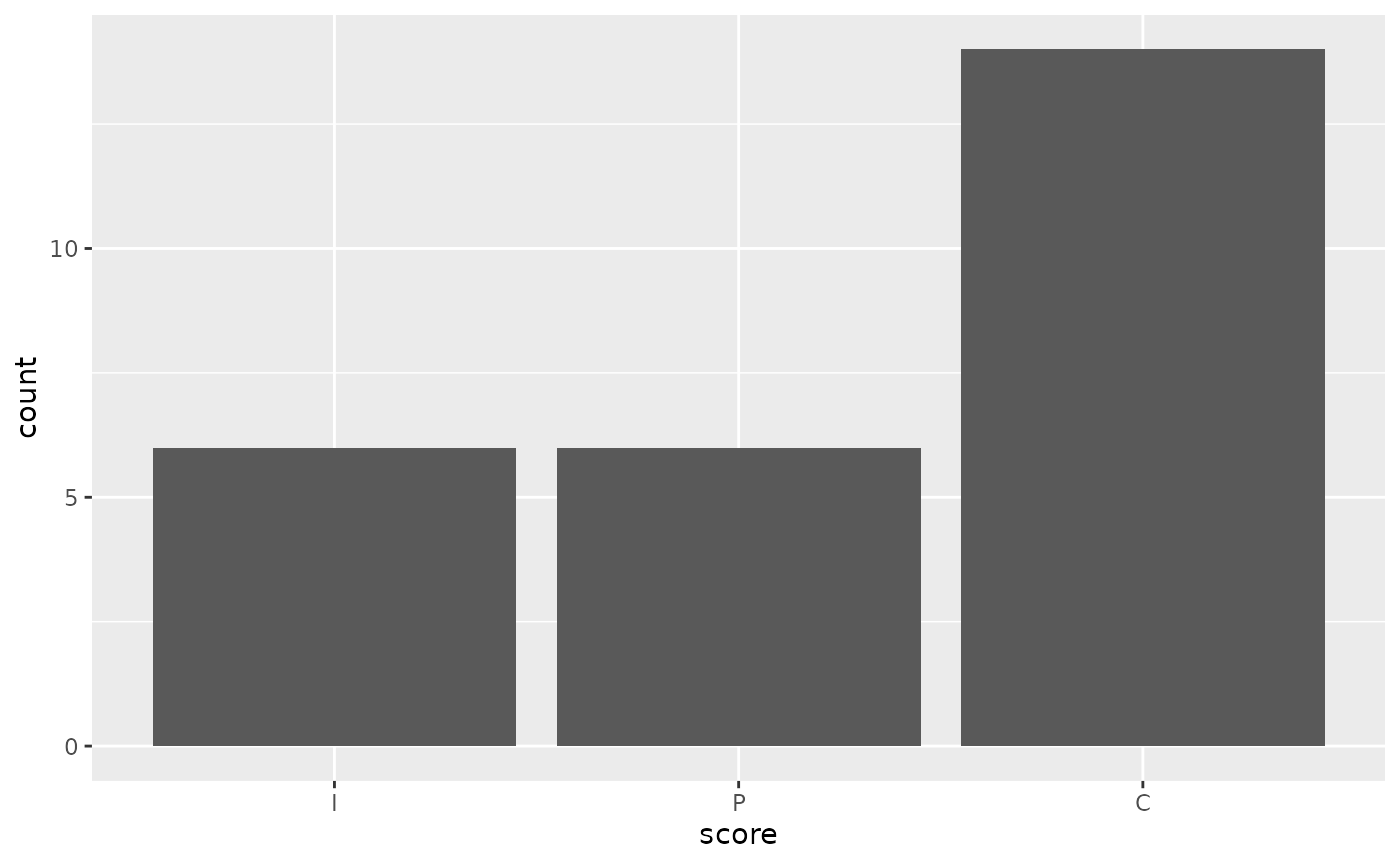

are_task_data |>
  ggplot() +
  aes(x = score) +
  geom_bar()

A ggplot2 bar plot, showing Claude was correct most of the time.

Claude answered fully correctly in 18 out of 29 samples, and partially correctly 4 times.For me, this leads to all sorts of questions:

Are there any models that are cheaper than Claude that would do just as well? Or even a local model?
Are there other models available that would do better out of the box?
Would Claude do better if I allow it to “reason” briefly before answering?
Would Claude do better if I gave it tools that’d allow it to peruse documentation and/or run R code before answering? (See btw::btw_tools() if you’re interested in this.)

These questions can be explored by evaluating Tasks against different solvers and scorers. For example, to compare Claude’s performance with OpenAI’s GPT-4o, we just need to clone the object and then run $eval() with a different solver chat:

are_task_openai <- are_task$clone()
are_task_openai$eval(solver_chat = chat_openai(model = "gpt-4o"))

Any arguments to solving or scoring functions can be passed directly to $eval(), allowing for quickly evaluating tasks across several parameterizations.

Using this data, we can quickly juxtapose those evaluation results:

are_task_eval <-
  vitals_bind(are_task, are_task_openai) |>
  mutate(
    task = if_else(task == "are_task", "Claude", "GPT-4o")
  ) |>
  rename(model = task)

are_task_eval |>
  mutate(
    score = factor(
      case_when(
        score == "I" ~ "Incorrect",
        score == "P" ~ "Partially correct",
        score == "C" ~ "Correct"
      ),
      levels = c("Incorrect", "Partially correct", "Correct"),
      ordered = TRUE
    )
  ) |>
  ggplot(aes(y = model, fill = score)) +
  geom_bar() +
  scale_fill_brewer(breaks = rev, palette = "RdYlGn")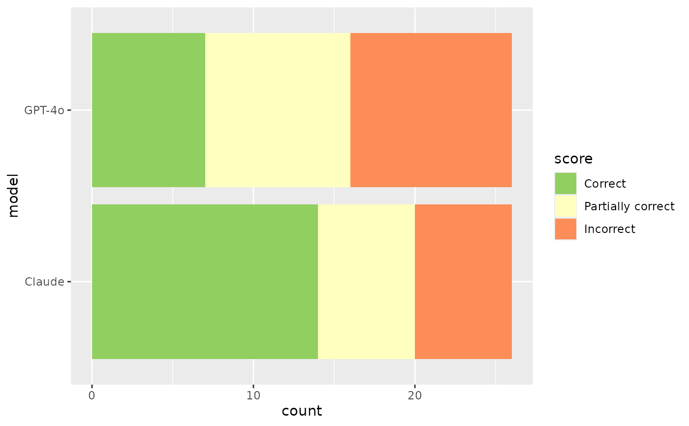

Is this difference in performance just a result of noise, though? We can supply the scores to an ordinal regression model to answer this question.

library(ordinal)

## 
## Attaching package: 'ordinal'

## The following object is masked from 'package:dplyr':
## 
##     slice

are_mod <- clm(score ~ model, data = are_task_eval)

are_mod

## formula: score ~ model
## data:    are_task_eval
## 
##  link  threshold nobs logLik AIC    niter max.grad cond.H 
##  logit flexible  58   -60.05 126.10 4(0)  3.53e-12 1.2e+01
## 
## Coefficients:
## modelGPT-4o 
##     -0.9443 
## 
## Threshold coefficients:
##     I|P     P|C 
## -1.7248 -0.3048

The coefficient for model == "GPT-4o" is -0.944, indicating that GPT-4o tends to be associated with lower grades. If a 95% confidence interval for this coefficient contains zero, we can conclude that there is not sufficient evidence to reject the null hypothesis that the difference between GPT-4o and Claude’s performance on this eval is zero at the 0.05 significance level.

confint(are_mod)

##                 2.5 %     97.5 %
## modelGPT-4o -1.967718 0.03831908

If we had evaluated this model across multiple epochs, the question ID could become a “nuisance parameter” in a mixed model, e.g. with the model structure ordinal::clmm(score ~ model + (1|id), ...).

This vignette demonstrated the simplest possible evaluation based on the are dataset. If you’re interested in carrying out more advanced evals, check out the other vignettes in this package!